My crypto-obsession from last year might have died down a little, but I still remain a long-term investor and a believer of decentralization. Moreover, it was predicting the crypto market’s next move that made dust off some of my old machine learning experiments and gave a fresh boost to my mission of becoming a data scientist. Though one could hardly hear me speak about this coin or that, I am still actively researching and building tools.
Tools like ShouldIHODL. It is an extremely simple website that does nothing else, but spit out a Yes or No to the question, of whether it is a good day to invest in Bitcoin or not. Emphasis on the word invest => buy for the longer term. I am not interested in sheer speculation, or the manipulated pump-and-dump schemes that flooded the markets last year. Also, it should go without saying that this is a simple side project built mainly for fun and learning purposes, and no financial advice of any kind. I don’t want to bear any responsibility for potential losses or missed opportunities on anyone’s behalf.

How does it work?
The raw data
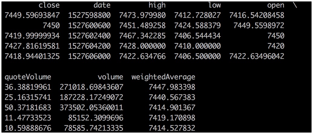
There is a fair bit of machine learning involved into the decision. First, a few tens of thousands of data points get fetched through the open Poloniex API. Each data point represents a 30-min interval from Bitcoin’s price history, containing data known from common charting tools and APIs:
open- price at the start of the intervalclose- price at the end of the intervallow- lowest price reached throughout the intervalhigh- the highest price reached throughout the intervalquoteVolume- volume movement expressed in units of the quote currency, a.k.a BTCbaseVolume- volume movement expressed in units of the base currency, either USD, EUR, or as in our case USDT
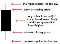
The first four are better known to chart enthusiasts and traders as what describes a candlestick:
 Photo: Investopedia
Cleaning up and extracting some features
The next step is taming the raw data into a Pandas DataFrame:

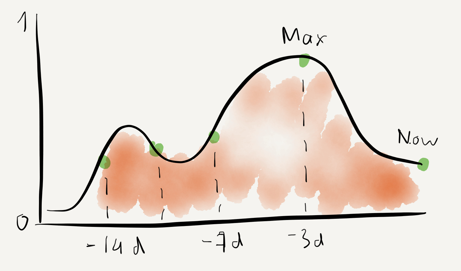
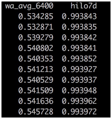
Having a few thousand candlesticks, one can use Pandas’ amazing rolling capabilities, in order to roll down HiLo ratios and moving averages normalized to the maximum in a given period:
num_periods_in_7d = 2 * 24 * 7 # Once, every 30 min

df['hilo_7d'] = df['low'].rolling(num_periods_in_7d).mean() /
df['high].rolling(num_periods_in_7d).mean()
# Still volatile, but less so than the current price
df['ma_30'] = df['avg_price'].rolling(30).mean()

# Reacting slowly to rapid changes. Can be used as a line of
# support / resistance
df['ma_6400'] = df['avg_price'].rolling(6400).mean()

# Gives an idea how far the average price is from a past peak,
# or if it is at the peak itself
df['ma_30_6400_ratio'] = df['ma_30'] /
df['avg_price'].rolling(6400).max()
Gather a few of those, and you will effectively have established a simple way of representing price patterns across a certain time window:

To save you further details, ratios like these are quite popular in technical analysis, and go under the name of “oscillators”. It has been proven that prices don’t just go wildly in one direction or another, but behave somewhat like forces in physics. An upward movement for instance, is caused by the force applied to the price by the buying group. It can’t go up indefinitely (even in crypto-land), but eventually faces a force of resistance which forces the price downward. That’s why after normalization, prices lines resemble sine waves and can be analyzed as such. For those of you interested in more technical analysis fundamentals, I would suggest getting familiar with the concepts of support and resistance.
Categorizing the cases
Based only on the inputs, how will our machine learning algorithm know which of them indicate a potential upward or downward movement? That’s right, we need to categorize them first. One simple way to do so, is to compare the price at any given time T with a price some time in the future (say, a week) - T'. If the price a week down the road is greater than the price at time T, we label the case as 1 (uptrend), or alternatively, as -1 (downtrend). Using Pandas’ forwards-and-backwards shifting function, this is a piece of cake:
# negative shifting will pair
df['future_price'] = df['ma_6400'].shift(-1 * num_periods_in_7d)

df['future_price_chg'] = (df['future_price'] / df['ma_6400']) - 1
df.loc[df['future_price_chg'] >= 0, 'label'] = 1
df.loc[df['future_price_chg'] <= 0, 'label'] = -1
Choosing a machine learning algorithm
Having extracted the features and labeled the data, our input matrix starts looking like a bunch of gibberish, but to the trained eye, and hopefully, to our machine learning algorithm it will be more than enough.

In the world of machine learning, there are many algorithms, each of which serving a different purpose. As much as media want you to believe in, ML is not all about neural nets. In fact, for the purposes of this project, I will use a decision tree classifier instead. Designed well, decision trees can be just as effective, at a fraction of the size and complexity of a decent neural network.
class sklearn.tree.DecisionTreeClassifier(criterion=’gini’,
                                          splitter=’best’,
                                          max_depth=None,
                                          min_samples_split=2,
                                          min_samples_leaf=1,
                                          min_weight_fraction_leaf=0.0,
                                          max_features=None,
                                          random_state=None,
                                          max_leaf_nodes=None,
                                          min_impurity_decrease=0.0,
                                          min_impurity_split=None,
                                          class_weight=None,
                                          presort=False)
Unlike deep NNs, decision trees have the advantage that they can be visualized easily. A decision tree graph can be exported and presented to a human expert who could confirm, if the branching criteria selected by the algorithm seems logical.

One disadvantage of decision trees is that they easily overfit, i.e. learn to solve the problem with the particular inputs at hand, but fail to really generalize the solution. All types of machine learning algorithm suffer from this, and there is really no single answer as to how to cope with it. One way is having your input data shuffled and split into two subsets. One goes for training the classifier, the other one for testing the accuracy of the algorithm:
from sklearn.model_selection import train_test_split
from sklearn.tree import DecisionTreeClassifier

inputs_train, inputs_test, labels_train, labels_test = train_test_split(inputs, labels)

tree_classifier = DecisionTreeClassifier()
tree_classifier.fit(inputs_train, labels_train)

# The testing data has not been fed to the estimator before
score = tree_classifier.score(inputs_test, labels_test)
While training, you can also introduce epoch-wise fitting using something like input data folding. Folding is a fancy name for splitting the original data set into a number of subsets, and deriving training and testing data points from each one:
from sklearn.model_selection import KFold
from sklearn.tree import DecisionTreeClassifier

tree_classifier = DecisionTreeClassifier()

for train_index test_index in KFold(n_splits=10, random_state=None, shuffle=False):
	X_train, Y_train = inputs.iloc[train_index], labels.iloc[train_index]
	X_test, Y_test = inputs.iloc[test_index], labels.iloc[test_index]

	tree_classifier.fit(inputs_train, labels_train)

	# This score relates to the particular subset only
	# You can yield it and average out the scores for all subsets
	# at then end. You can also fit each subset into a new tree.
	# When predicting the overall score, all trees need to be called,
	# and the results of their scores averaged out.
	score = tree_classifier.score(inputs_test, labels_test)
Note on Random Forests
Another, perhaps even better option is to use random forests. A random forest is a collection of trees, generated using randomized hyperparameters (max depth, min split count, max number of leaf nodes, etc), to each of which different inputs are fed. When predictions are derived, each tree is asked to predict a result separately, and the majority vote is taken:
 Source: Wikimedia
A random forest is trained and tested in pretty much the same way as a single decision tree:
from sklearn.ensemble import RandomForestClassifier
from sklearn.model_selection import cross_val_score

# An important parameter here is the number of trees in the forest
tree_classifier = RandomForestClassifier(n_estimators=50)

# Cross-val-score combines folding, splitting, and scoring in one function
score = cross_val_score(tree_classifier, X=inputs, y=labels, cv=10).mean()
No matter how you approach it, once trained, the classifier can be used for predicting the outcome of a future event, by feeding it with current pricing data (transformed into input features, of course):
current_point_as_inputs = extract_inputs_from_data_frame(df.iloc[-1]))

# This call will return either `1` or `-1` (our labels)
end_class = tree_classifier.predict(current_point_as_inputs)

# This call will return an array of probabilities for each class to occur
class_probs = tree_classifier.predict_proba(current_point_as_inputs)
# class_probs => [0.23, 0,77]
Rendering the outputs and scheduling daily updates
Having made our classifier output a decision, it is time to display it to visitors of the website. Since this entire operation is being read from and hosted on GitHub, I am using the magic of Travis to fetch and transform historical data, feed it through a decision tree classifier, and render the output using a static site generator for Python, called Pelican. Travis supports scheduled corn rebuilds of a certain branch which are ideal for my purpose. So, in essence, I’m doing all of this using pretty much using only a crown job, and some GitHub disk space for storing the rendered outputs. Let’s talk about serverless architecture, shall we? 😀
What is in it for me?
Nothing. I am neither planning to profit from the website, nor to collect user data or track user behavior. At the moment, I am doing this only for learning, and personal development purposes. Everyone is allowed to check out the site, as well as the code, leave comments, posts suggestions and pull requests. As mentioned at the beginning of the article, this tool is not a professional trading advice, and basing your trading decisions solely on what it shows you, will be equal to spending your money on the national lottery (which many of you do, but still).
Enjoy, and don’t hesitate to leave me feedback, or share the word on Twitter with your friends.

Leave a comment